Dilemma in Model Pruning: Effective or Efficient?
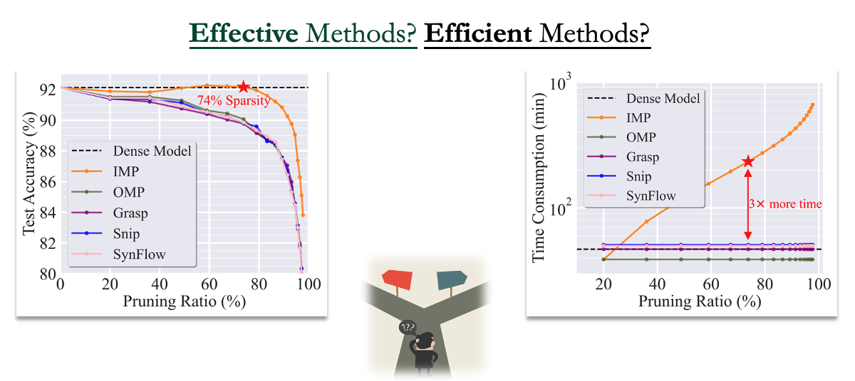
Among the many powerful pruning methods, Iterative Magnitude Pruning (IMP) is one of the most significant and popular methods, which prunes the model in an iterative manner and can reach an extremely sparse level without any performance loss. However, it often consumes much more than training a dense model from scratch. In contrast, efficient one-shot pruning methods can not deliver a high-quality sparse subnetwork, as shown in Figure 1. Therefore, existing pruning methods have reached a dilemma over choosing between the effective method and the efficient method.

Model Pruning as a Bi-level Optimization Problem
We start our research by revisiting the model pruning problem and reformulating it to a bi-level optimization (BLO) problem:
\[\min_{\mathbf{m} \in \mathcal{S}} \ell(\mathbf{m} \odot \boldsymbol\theta^{\ast}(\mathbf{m})) \quad \quad \text{subject to} \,\,\, \boldsymbol\theta^{\ast}(\mathbf{m}) = \text{argmin}_{\boldsymbol\theta \in \mathbb{R}^n}\, \ell(\mathbf{m} \odot \boldsymbol\theta + \frac{\gamma}{2}\|\boldsymbol\theta\|_2^2),\]where the upper-level problem optimizes the pruning mask for the model and the lower-level retrains the model with the fixed mask. The benefits from this bi-level formulation are two-folded.
-
First, we have the flexibility to use the mismatched pruning and retraining objectives.
-
Second, the bi-level optimization enables us to explicitly optimize the coupling between the retrained model weights and the pruning mask through the implicit gradient (IG)-based optimization routine.
Optimization Foundation of BIP
BLO is different from other optimization problems, as the gradient descent of the upper-level variable will involve the calculation of the implicit gradient (IG):
\[\frac{d\ell(\mathbf{m}\odot\boldsymbol\theta^\ast(\mathbf{m}))}{d\mathbf{m}} = \nabla_{\mathbf{m}}\ell(\mathbf{m}\odot\boldsymbol\theta^\ast(\mathbf{m})) + \frac{d{\boldsymbol\theta^\ast(\mathbf{m})}^\top}{d\mathbf{m}} \nabla_{\boldsymbol\theta}\ell(\mathbf{m}\odot\boldsymbol\theta^\ast(\mathbf{m})).\]The IG challenge is a fingerprint of the BLO solver and derives from the implicit function theory. It refers to the gradient of the lower-level solution w.r.t. the upper-level variable and in most cases is very difficult to calculate. The main reason is it usually involves the second-order derivative and matrix inversion:
\[\frac{d{\boldsymbol\theta^\ast(\mathbf{m})}^\top}{d\mathbf{m}} = -\nabla^2_{\mathbf{m}\boldsymbol\theta}\ell(\mathbf{m}\odot\boldsymbol\theta^\ast)[\nabla^2_{\boldsymbol\theta}\ell(\mathbf{m}\odot\boldsymbol\theta^\ast) + \gamma \mathbf{I}]^{-1}.\]Very luckily, in the model pruning scenario, the upper- and lower-level variables are always combined as bi-linear variables. We can thus leverage this bi-linear property and derive a closed-form IG solution, which only requires the first-order derivative:
\[\frac{d{\boldsymbol\theta^\ast(\mathbf{m})}^\top}{d\mathbf{m}} = -\frac{1}{\gamma} \text{diag}(\nabla_{\mathbf{z}}\ell(\mathbf{z})|_{\mathbf{z} = \mathbf{m} \odot \boldsymbol\theta^\ast}).\]This also makes our later proposed bi-level pruning algorithm a purely first-order method.
BiP: Bi-level Optimization-based Pruning
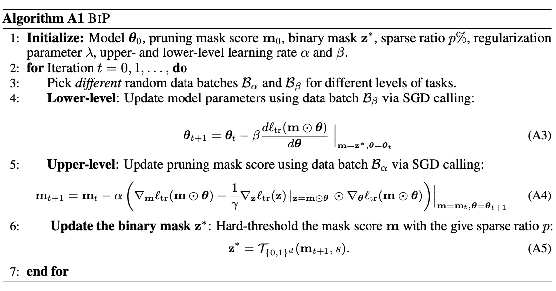
We propose our bi-level pruning algorithm (BiP). We adopt the alternating optimization procedure by updating the upper- and lower-variable in turn.

More details of BiP
We show the illustration of the BiP algorithm in Figure 3 below. We start with a pretrained model and some mask initialization. For the lower level, we use stochastic gradient descent to update the model parameter with the fixed mask. For the upper level, as the mask is supposed to contain either 0 or 1, representing whether a parameter should be removed or retained, we first relax the “binary” masking “variables” to “continuous” masking “scores”, which can be updated with auto-differentiation in most of the deep learning algorithms. In the forward path, we project the scores onto the discrete constraint using hard thresholding, where the top k elements are set to 1s and the others to 0s. Thus, we summarize our upper-level problem as stochastic projected gradient descent, in short SPGD.

Comparison to IMP and OMP
We also show the illustration of the iterative magnitude pruning (IMP) and one-shot magnitude pruning (OMP) below for comparison.


Experiment results
BIP identifies high-accuracy subnetworks in unstructured pruning
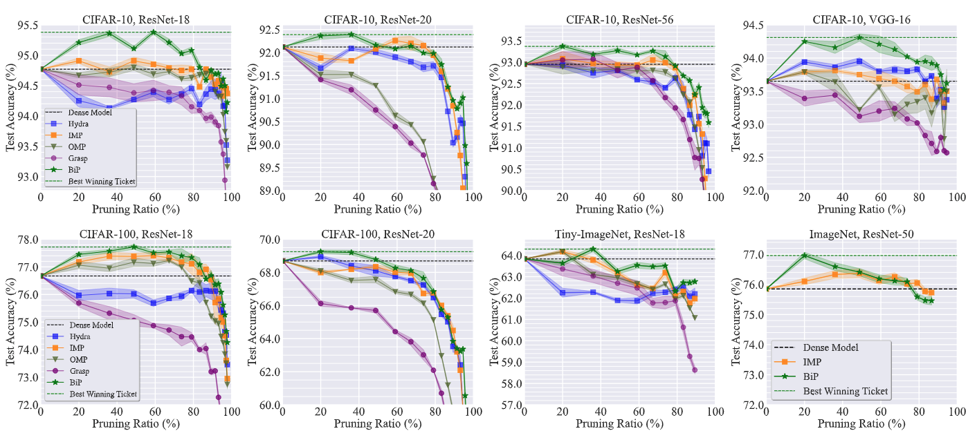
In Figure 6 below, we show the unstructured pruning trajectory (given by test accuracy vs. pruning ratio) of BIP and baseline methods in 8 model-dataset setups. BiP outperforms its baselines in nearly all the settings and also finds the sparsest winning tickets nearly every time. For some settings like CIFAR-10 with model VGG-16, BiP is even capable of finding winning tickets with a pruning ratio over 90%

BIP identifies high-accuracy subnetworks in structured pruning
A similar phenomenon can be observed in the structured pruning setting as well.

BiP achieves high pruning efficiency.
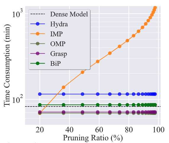
Next, we show the high efficiency of BiP compared to the state-of-the-art IMP method [1]. As we have longed for, BiP consumes sparsity-agnostic time consumptions just like the one-shot pruning methods and can be 3~7 times faster than IMP.

BiP requires no rewinding.
Another advantage of BIP is that it insensitive to model rewinding to find matching subnetworks. Recall that rewinding is a strategy used in Lottery Ticket Hypothesis [2] to determine what model initialization should be used for retraining a pruned model. In Figure 9, we show the test accuracy of the BIP-pruned model when it is retrained at different rewinding epochs under various datasets and model architectures. As we can see, a carefully-tuned rewinding scheme does not lead to a significant improvement over BIP without retraining. This suggests that the subnetworks found by BIP are already of high quality and do not require any rewinding operation.

Citation
1
2
3
4
5
6

@inproceedings{zhang2022advancing,
  title = {Advancing Model Pruning via Bi-level Optimization},
  author = {Zhang, Yihua and Yao, Yuguang and Ram, Parikshit and Zhao, Pu and Chen, Tianlong and Hong, Mingyi and Wang, Yanzhi and Liu, Sijia},
  booktitle = {Advances in Neural Information Processing Systems},
  year = {2022}
}
Reference
[1] Xiaolong Ma et al. “Sanity Checks for Lottery Tickets: Does Your Winning Ticket Really Win the Jackpot?” NeurIPS 2021.
[2] Jonathan Frankle et al. “The Lottery Ticket Hypothesis: Finding Sparse, Trainable Neural Networks.” ICLR 2019.